Creating an Avatar

When I first looked over the extra credit assignments and saw the Avatar tab I was nervous.  How do I, the not so computer savvy guy, create an avatar?  I was dreading the thoughts I had of a laborous event.  I held off on starting this project until a few weeks into the semester.

Today I saw that a fellow student in the class had done their blog on creating an avatar and saw how easy it actually was.  I went to the site they had recommended, IMVU, and began the intial creation of my avatar.  After about 30 minutes I realized I was struggling a bit to get my changes to take on my avatar.   I thought  that this avatar looked more life like, but maybe there is a more user friendly site. 

After searching through the recommended sites I came across http://www.meez.com/ .  This site was easy to set up a new account and get started.  All I had to do was create an account, enter my personal information, and finally give my email address. 

Click Join Now

Select Your Avatar

Enter Personal Information

Logged In and Ready to Adapt Avatar to My Image

Once logged in I was able to adapt my avatar to look like me.  It was very simple and only took 15 minutes to change my hairstyle to bald, change my shirt to something that matches my style, and then click save to ensure all my work was properly updated.  The five tabs across the top appropriately labeled for what they do are a simple click and update to make changes.  The search block is also helpful on this site.

Here is my self image on my avatar, Philfe1.  I will definitely refer others trying to do an avatar to this simple website.

Me in Avatar Form

How to Insert A Simple Filter on Excel

After last week's exciting Pivot Table instructions I thought it might be a good time to show everyone a simple step that allows a database manager quick access to raw numbers.  I think the "Filter" tool is the most helpful thing in Excel in my day to day life as a Logistics Manager and HR guy when using Excel.  I can get the raw number fast to do projections on ordering and meeting the needs of my everchanging career.

I have created an extremely simple database that you will see below in a screen shoot.  It has three headings where I will install the previously mentioned filter.  These headings are labeled Group, Name, and Size Shirt.  Under these headings I filled in information that would be input on data gathering for this database.  Here is the initial screen shot.

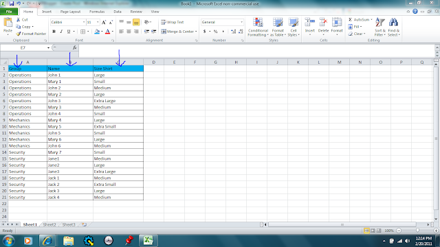
Intial Data Entry with Group Labels (See Arrows)

 Now that I have the data I need to track I would like to simplify it into only Operations members that need a large shirt.  That may be easy to simply count with only 20 names in this example but dealing with 400-450 people as I do daily I need a tool to help. I am going to put a simple filter on the group headings to make this task extremely easy. 

First go to the "Data" heading on the top of the Excel database and click on it.  Here is what the screen should look like.

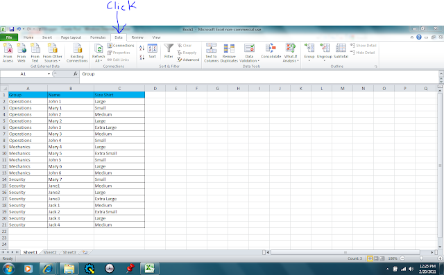
Going to Data Tab in Excel

Next highlight A1-C1, the group headings.  Now we can install the filter for the groupings.  Simply click on the "Filter" button that looks like a funnel.  Here is what it will look like with a filter on the groupings.



Filter Applied By Highlighting Heading & Clicking on Filter

Now that we have a filter let's use it.  Move your mouse over the "Group Heading"  to the filter icon.  Select Operations out of the group. Click Okay and Excel will allow only the Operations information to show. 



Using the Filter to Narrow Your Data

 With the first filter applied, Operations, I am going to apply only large sizes next.

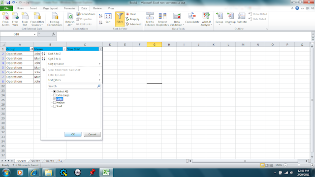
Further Filtering to Meet Needs

Now that we have filtered by group and size I can see that there only two people that need a size large in Operations.  Note the small print at the bottom of the next screen capture.  When each filter is applied it will tell you how many records meet your criteria. There are seven total in Operations and two for size large.

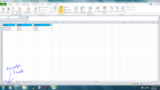
Fully Filtered Data

This is a really simple way to get a quick number of items without having to a Pivot Table in my opinion.  I actually used filtering during my previous work week to report how many people needed uniforms and their sizes.  I was able to give my direct supervisor a quick overall number based on sizes needed to be ordered and also did do a Pivot Table to make the presentation of the database nicer.  My supervisor likes the filtering because he can filter through any of the twenty functional groups we have in our area in mere seconds.

I hope this simple tool is useful to you in your daily uses of Excel.

Excel Project

ExcelProject-12February2011

Today I am tying up the loose ends of this week’s Excel project in ISM 3004.  I am going through a step by step process to provide you, my blog follower, with a simple set of instructions of how to create a basic pivot table.  We will take a peek at the “Raw Data” used to make the pivot table first.  Next we will discuss the inputs required to make the table work.  Finally we will see the end product, the “AvgIncrease” pivot table.

The “Raw Data” is a listing of 500 individuals heart rates based on age and gender.  We take this data seen below and insert it into the pivot table by using the “Insert Tab” and select Pivot Table.  This data has been manipulated and formatted to fit the desires of a fictitious gym owner.

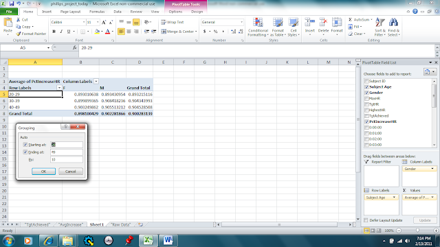
The next page that will open is a new tab on Excel.  I then manipulate the table to fit my data needs. The owner wants to see the percent of increase grouped by age and gender.  Here is a peak at how I will set up the columns, rows, and formatting to make it work.  Look at the right side of the screen shot to see the exact details on how to make the project work.

Now that you see the inputs for row labels are the subject age and the column labels are gender.  The values used are the average increase in heart rate in which I formatted as an average.  This will allow me to have a nice clean average when I format age in groups of ten, 20-29 etc.  I will do the formatting in those groups by right clicking on 20-20 in the row column, click on grouping, and then set the “By:” to “10”

Next we will meet the owner’s requirement of showing the results in percentages and blocking the Grand Total Labels.  Highlight the data in B:5/C:5-B:7-C:7, right click and then select format.  Next select percentage and ensure there is only one decimal place. The last step is to right click on both “Grand Total” headings and then click remove “Grand Total” to finish the pivot table. Here is the view of the pivot table and I hope my instructions will help others in their attempts at completing a pivot table